Legacy data formats with cloud tools • earthdatalogin

Not all data formats which NASA EarthData makes available on cloud storage are provided in cloud-optimized or even VSI-compatible formats. A stark example is HDF4. Here we illustrate how to work with these data formats while staying as close to the cloud-native workflow shown in other vignettes.

Aside: note that in many cases, these same data products may be available in cloud-native formats from other providers. Particular to the example here, see the cloud-optimized MODIS catalog on the Planetary Computer STAC.

library(earthdatalogin)

library(rstac)
library(gdalcubes)
library(spData)
library(sf)
gdalcubes_options(parallel = TRUE)

CA <- spData::us_states |> dplyr::filter(NAME=="California")
bbox <- CA |> st_bbox()
start <- "2022-01-01"
end <- "2022-12-31"

items <- stac("https://cmr.earthdata.nasa.gov/stac/LPCLOUD") |> 
  stac_search(collections = "MOD13Q1.v061",
              bbox = c(bbox),
              datetime = paste(start,end, sep = "/")) |>
  post_request() |>
  items_fetch()
#> 
  |                                                                                                                                                                                                                                                                
  |==========================================================================================================================================================================================================================================================| 100%

HDF4 doesn’t support cloud (range-request-based) access / VSI. Instead, we download all matching assets with earthdatalogin authentication:

paths <- items$features |>
  purrr::map(list("assets", "data", "href")) |> 
  unlist() |>
  purrr::map_chr(edl_download)

Rather than create an image collection using STAC metadata, we can use the recognized format and the local paths:

paths <- fs::dir_ls(".", glob="*.hdf")
col <- gdalcubes::create_image_collection(paths, format = "MxD13Q1")

# Define whatever view you like!
v = cube_view(srs = "EPSG:4326",
              extent = list(t0 = as.character(start), 
                            t1 = as.character(end),
                            left = bbox[1], right = bbox[3],
                            top = bbox[4], bottom = bbox[2]),
              nx = 512, ny = 512, dt = "P1M")

raster_cube(col, v) |> 
  select_bands("NDVI") |> 
  animate(col = viridisLite::mako, fps=2, 
          save_as="img/ndvi.gif")
#> [1] "/home/cboettig/boettiger-lab/earthdatalogin/inst/vignette-sources/img/ndvi.gif"

library(tmap)
r <- 
  raster_cube(col, v) |> 
  select_bands("NDVI") |> 
  st_as_stars.cube()

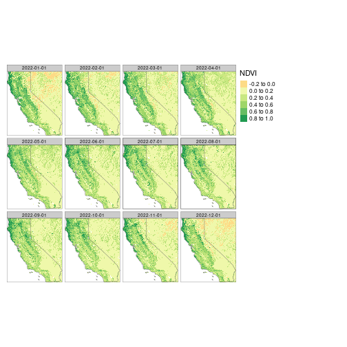
tm_shape(r) + tm_raster("NDVI") +
  tm_shape(CA) + tm_borders()

plot of chunk india_ndvi_modis