Programmatic Access from R & Python

The MCP server speaks streamable HTTP, so you can call its tools from any language — no LLM client required. You can also wire the tools into an LLM agent so the model writes and runs queries on its own.

This page works one real example three ways, in both R and Python:

Local compute — a DuckDB on your own machine, no server involved.
The MCP server — the same pipeline, executed next to the data.
MCP and a chat model — hand the question to an LLM and let it work.

You never have to write SQL: dbplyr and ibis compile it for you, and the server will happily run what they produce.

Full runnable scripts are in the examples/ folder.

A worked example: birds and income in New Haven

Everything below answers one question:

In each census tract of New Haven, Connecticut, how many bird observations are there, and how does that track median household income?

It needs three datasets that were never designed to be used together:

Dataset	What we take from it
GBIF occurrences (`gbif-derived`)	every record with `class = 'Aves'`
ACS 2020–2024 block groups (`us-census`)	`MHHI` and `TotPop`, plus each block group's tract
Census 2024 places (`us-census`)	the footprint of the city of New Haven

Normally that means three reprojections and two point-in-polygon joins. Here it doesn't, because all three are published on the same H3 hex grid: every row carries h0…h10 columns naming the hex cell it falls in. "Which tract is this bird in?" becomes a key equality — an ordinary join on h10.

Two columns do the work. h10 (~0.015 km²) is the join key, fine enough that a cell rarely straddles two city block groups. h0 (whole-continent cells) is the partition column: both datasets are stored one file per h0, so including it in the join lets DuckDB skip all but one file per dataset. Always join on both. GBIF's h0 file for the US Northeast alone is 22 GB and 525 M rows.

Read paths from the catalog, not from here

The S3 paths below are copied from get_stac_details. Always do that rather than typing paths from memory — see Available Datasets.

The answer looks like this:

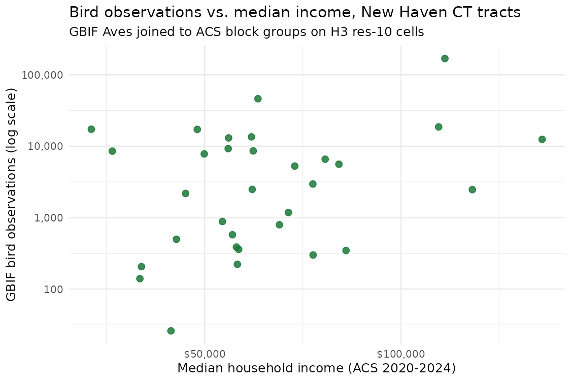
Bird observations against median household income for the 32 census tracts of New Haven CT, showing a wide scatter with a weak upward tilt

Across New Haven's 32 tracts, observation counts span more than three orders of magnitude (26 to 169,062) against a sixfold income range ($21k–$136k). The tilt is upward but weak — Pearson r = 0.33 against log counts, Spearman ρ = 0.23 — and a handful of hotspots dominate everything: the top tract is East Rock Park. So there is a hint of the "luxury effect" reported in the urban-ecology literature, but on this evidence recorded birds mostly track birders, not income and not people (population does even worse, r = 0.20). Sampling bias like that is the first thing to reckon with in any analysis built on opportunistic occurrence data.

1. Local compute

No server involved. A DuckDB running on your own machine reads Parquet straight out of the source.coop mirror, and your dplyr or ibis code is compiled to SQL and executed inside that engine. Only the final 32-row answer is ever materialised.

R — dplyr and duckdbfs

duckdbfs handles the connection and dbplyr compiles your dplyr verbs into DuckDB SQL, so filters, joins and aggregations all run inside the engine.

library(duckdbfs)
library(dplyr)

# Anonymous reads from the source.coop mirror on AWS us-west-2. The bucket name
# contains dots, so path-style addressing is required for the TLS cert to match.
duckdb_s3_config(
  s3_endpoint  = "s3.us-west-2.amazonaws.com",
  s3_region    = "us-west-2",
  s3_url_style = "path",
  s3_use_ssl   = TRUE,
  anonymous    = TRUE
)

# Keep a laptop-sized footprint: DuckDB streams and spills to disk rather than
# trying to hold the join in RAM.
#
# Spill to node-local scratch, not the working directory. On JupyterHub, HPC or
# any cluster, $HOME is networked storage and spilling there is far slower than
# the local ephemeral disk that tempdir() resolves to.
duckdb_config(
  memory_limit   = "3GB",
  temp_directory = file.path(tempdir(), "duckdb")
)

open_dataset() globs the h0=* partitions under each prefix and returns a lazy dplyr table.

base <- "s3://us-west-2.opendata.source.coop/cboettig"

places      <- open_dataset(paste0(base, "/census/census-2024/place/hex"))
blockgroups <- open_dataset(paste0(base, "/census/acs-2020-2024/blockgroup/hex"))
gbif        <- open_dataset(paste0(base, "/gbif/2026-06/hex"))

Now the analysis — plain dplyr, start to finish:

# 1. The res-10 cells that make up the city of New Haven.
nh_cells <- places |>
  filter(STATEFP == "09", NAME == "New Haven") |>
  distinct(h0, h10)

# 2. Connecticut block groups falling inside those cells, tagged with their
#    11-digit tract id (state + county + tract).
nh_bg <- blockgroups |>
  filter(STATEFP == "09") |>
  semi_join(nh_cells, by = c("h0", "h10")) |>
  mutate(tract = paste0(STATEFP, COUNTYFP, TRACTCE))

# 3. A cell -> tract lookup. min() breaks ties so a cell straddling a boundary
#    is counted once rather than in both tracts.
cell_tract <- nh_bg |>
  group_by(h0, h10) |>
  summarise(tract = min(tract), .groups = "drop")

# 4. Income and population per tract. Both are block-group attributes repeated
#    on every hex row, so deduplicate by block group first.
tract_stats <- nh_bg |>
  distinct(tract, GEOID, TotPop, MHHI) |>
  group_by(tract) |>
  summarise(
    population = sum(TotPop, na.rm = TRUE),
    # A median is not a sum: to roll block groups up to a tract, take the
    # population-weighted mean of their medians. Block groups whose income
    # estimate is suppressed drop out of both halves of the ratio.
    median_income = sum(MHHI * TotPop, na.rm = TRUE) /
      sum(ifelse(is.na(MHHI), 0, TotPop), na.rm = TRUE),
    .groups = "drop"
  )

# 5. Bird observations per tract.
birds <- gbif |>
  filter(class == "Aves") |>
  inner_join(cell_tract, by = c("h0", "h10")) |>
  count(tract, name = "bird_observations")

result <- tract_stats |>
  inner_join(birds, by = "tract") |>
  arrange(desc(bird_observations))

result |> show_query()   # inspect the DuckDB SQL dbplyr wrote for you
tracts <- collect(result)   # ~13 s; only these 32 rows come back to R

library(ggplot2)

ggplot(tracts, aes(median_income, bird_observations)) +
  geom_point(size = 2.6, alpha = 0.85, colour = "#1b7837") +
  scale_y_log10(labels = scales::comma) +
  scale_x_continuous(labels = scales::dollar) +
  labs(x = "Median household income (ACS 2020-2024)",
       y = "GBIF bird observations (log scale)") +
  theme_minimal(base_size = 12)

Python — ibis

ibis is the Python counterpart to dbplyr: deferred expressions that compile to DuckDB SQL, with nothing executed until .execute(). The pipeline below is a line-for-line translation of the R one.

python

import tempfile

import ibis
from ibis import _

# Extensions and DuckDB settings go straight into connect(), the rough
# counterpart of duckdb_s3_config() + duckdb_config() on the R side. mkdtemp()
# spills to node-local scratch rather than a networked $HOME.
con = ibis.duckdb.connect(
    extensions=["httpfs"],
    memory_limit="3GB",
    temp_directory=tempfile.mkdtemp(prefix="duckdb-"),
)
con.raw_sql("""
    CREATE SECRET source_coop (
        TYPE S3, KEY_ID '', SECRET '',
        ENDPOINT 's3.us-west-2.amazonaws.com', REGION 'us-west-2',
        URL_STYLE 'path', USE_SSL 'true',
        SCOPE 's3://us-west-2.opendata.source.coop'
    )""")

BASE = "s3://us-west-2.opendata.source.coop/cboettig"

def hexed(path: str) -> ibis.Table:
    # con.sql() keeps the path inline; con.read_parquet() would register a
    # named view, like open_dataset() in R.
    return con.sql(f"SELECT * FROM read_parquet('{BASE}{path}')")

places      = hexed("/census/census-2024/place/hex/h0=*/data_0.parquet")
blockgroups = hexed("/census/acs-2020-2024/blockgroup/hex/h0=*/data_0.parquet")
gbif        = hexed("/gbif/2026-06/hex/h0=*/data_0.parquet")

python

# 1. The res-10 cells that make up the city of New Haven.
nh_cells = (
    places.filter(_.STATEFP == "09", _.NAME == "New Haven")
    .select("h0", "h10")
    .distinct()
)

# 2. Connecticut block groups inside those cells, tagged with their tract id.
nh_bg = (
    blockgroups.filter(_.STATEFP == "09")
    .semi_join(nh_cells, ["h0", "h10"])
    .mutate(tract=_.STATEFP + _.COUNTYFP + _.TRACTCE)
)

# 3. A cell -> tract lookup, with ties broken so cells are counted once.
cell_tract = nh_bg.group_by(["h0", "h10"]).agg(tract=_.tract.min())

# 4. Income and population per tract, deduplicated by block group first. A
#    median is not a sum, so roll up as a population-weighted mean.
tract_stats = (
    nh_bg.select("tract", "GEOID", "TotPop", "MHHI")
    .distinct()
    .group_by("tract")
    .agg(
        population=_.TotPop.sum(),
        median_income=(_.MHHI * _.TotPop).sum()
        / _.MHHI.isnull().ifelse(0, _.TotPop).sum(),
    )
)

# 5. Bird observations per tract. `class` is a Python keyword, so index it.
birds = (
    gbif.filter(_["class"] == "Aves")
    .inner_join(cell_tract, ["h0", "h10"])
    .group_by("tract")
    .agg(bird_observations=_.count())
)

result = tract_stats.inner_join(birds, "tract").order_by(_.bird_observations.desc())

print(ibis.to_sql(result))   # inspect the DuckDB SQL ibis wrote for you
tracts = result.execute()    # ~9 s; only these 32 rows come back to Python

2. The MCP server

The local route pulled 169 MiB across the network to answer with 32 rows. The MCP server sits next to the data, so it can run the same scan there and send back only the answer — and you need nothing installed but an HTTP client.

You still do not write SQL. dbplyr and ibis already compiled your pipeline; sql_render() and ibis.to_sql() hand you that string, and the server's query tool runs it.

R — dplyr, executed on the server

Only two things change from the local version. First, build the tables from read_parquet() rather than open_dataset(). open_dataset() registers a DuckDB view, so dbplyr renders FROM <view name> — which means nothing to a server that has no such view. Keeping the path inline makes the generated SQL portable:

# The server reads the NRP copy, so these are the NRP paths the catalog
# publishes. dbplyr only needs column NAMES to compile the query, and gets them
# by reading Parquet footers -- a fraction of a second, not a scan.
duckdb_s3_config(s3_endpoint = "s3-west.nrp-nautilus.io",
                 s3_url_style = "path", s3_use_ssl = TRUE, anonymous = TRUE)
con <- cached_connection()

hex <- function(path) {
  tbl(con, sql(paste0("SELECT * FROM read_parquet('s3://public", path, "')")))
}

places      <- hex("-census/census-2024/place/hex/h0=*/data_0.parquet")
blockgroups <- hex("-census/acs-2020-2024/blockgroup/hex/h0=*/data_0.parquet")
gbif        <- hex("-gbif/2026-06/hex/h0=*/data_0.parquet")

The dplyr pipeline itself is byte-for-byte identical — steps 1–5 above, unchanged. Only the last line differs: render instead of collect, and post.

library(httr2)
library(jsonlite)

mcp_url <- "https://duckdb-mcp.nrp-nautilus.io/mcp"

mcp_call <- function(name, arguments) {
  resp <- request(mcp_url) |>
    req_headers(Accept = "application/json, text/event-stream",
                `Content-Type` = "application/json") |>
    req_body_json(list(jsonrpc = "2.0", id = 1L, method = "tools/call",
                       params = list(name = name, arguments = arguments))) |>
    req_timeout(600) |>
    req_perform()

  body <- resp_body_string(resp)
  if (grepl("event-stream", resp_content_type(resp), fixed = TRUE)) {
    data <- sub("^data: ", "", grep("^data: ", strsplit(body, "\n")[[1]], value = TRUE))
    out <- fromJSON(data[length(data)], simplifyVector = FALSE)
  } else {
    out <- fromJSON(body, simplifyVector = FALSE)
  }
  if (!is.null(out$error)) stop(out$error$message)
  out$result$content[[1]]$text
}

sql <- as.character(sql_render(result))   # <- dplyr, compiled to DuckDB SQL
tracts <- mcp_call("query", list(sql_query = sql)) |>
  parse_md_table() |>
  mutate(across(c(population, median_income, bird_observations), as.numeric))

query answers with a markdown table; parse_md_table() (in the full script) is a dozen lines of strsplit. Keep every column character on the way back — tract ids are FIPS codes, and as.numeric() would eat their leading zero.

Python — ibis, executed on the server

The same two changes: repoint the tables at NRP, then render instead of execute.

python

from mcp import ClientSession
from mcp.client.streamable_http import streamable_http_client

MCP_URL = "https://duckdb-mcp.nrp-nautilus.io/mcp"

def hexed(path: str) -> ibis.Table:
    return con.sql(f"SELECT * FROM read_parquet('s3://public{path}')")

# ... the pipeline is unchanged ...

async def main():
    sql = str(ibis.to_sql(result))   # <- ibis, compiled to DuckDB SQL
    async with streamable_http_client(MCP_URL) as (read, write):
        async with ClientSession(read, write) as session:
            await session.initialize()
            out = await session.call_tool("query", {"sql_query": sql})
    tracts = parse_md_table(out.content[0].text)

WARNING

streamable_http_client is the mcp 2.x name and yields two streams. On the 1.x SDK it is streamablehttp_client and yields a third element, the session id.

Without dplyr or ibis

If you just want to run SQL and skip the dplyr/ibis layer, the query tool is one HTTP POST.

R

The same call in R. No R MCP client speaks HTTP directly (mcptools is stdio-only — see the ellmer + mcptools section below). The server runs in stateless mode, so you can hit the JSON-RPC endpoint directly with httr2. Responses arrive as server-sent events (SSE).

library(httr2)
library(jsonlite)

mcp_url <- "https://duckdb-mcp.nrp-nautilus.io/mcp"

sql <- "
SELECT country, name_en, subtype
FROM read_parquet('s3://public-overturemaps/2026-02-18.0/countries.parquet')
WHERE subtype = 'country' AND is_land
ORDER BY name_en
LIMIT 10
"

parse_sse <- function(body) {
  lines <- strsplit(body, "\n", fixed = TRUE)[[1]]
  data_lines <- sub("^data: ", "", lines[grepl("^data: ", lines)])
  lapply(data_lines, fromJSON, simplifyVector = FALSE)
}

mcp_call <- function(method, params, id = 1L) {
  resp <- request(mcp_url) |>
    req_headers(
      Accept = "application/json, text/event-stream",
      `Content-Type` = "application/json"
    ) |>
    req_body_json(list(
      jsonrpc = "2.0",
      id = id,
      method = method,
      params = params
    )) |>
    req_perform()

  body <- resp_body_string(resp)
  ctype <- resp_content_type(resp)
  if (grepl("event-stream", ctype, fixed = TRUE)) {
    msgs <- parse_sse(body)
    msgs[[length(msgs)]]
  } else {
    fromJSON(body, simplifyVector = FALSE)
  }
}

resp <- mcp_call("tools/call", list(
  name = "query",
  arguments = list(sql_query = sql)
))

for (block in resp$result$content) {
  cat(block$text, "\n")
}

Python

The official mcp SDK speaks streamable HTTP natively.

bash

pip install mcp

python

import asyncio
from mcp import ClientSession
from mcp.client.streamable_http import streamable_http_client

MCP_URL = "https://duckdb-mcp.nrp-nautilus.io/mcp"

SQL = """
SELECT country, name_en, subtype
FROM read_parquet('s3://public-overturemaps/2026-02-18.0/countries.parquet')
WHERE subtype = 'country' AND is_land
ORDER BY name_en
LIMIT 10
"""

async def main():
    async with streamable_http_client(MCP_URL) as (read, write):
        async with ClientSession(read, write) as session:
            await session.initialize()

            tools = await session.list_tools()
            print("Available tools:", [t.name for t in tools.tools])

            result = await session.call_tool("query", {"sql_query": SQL})
            for block in result.content:
                print(block.text)

asyncio.run(main())

Local or server?

Both routes ran the identical query and returned the identical 32 rows.

	Local DuckDB (source.coop)	MCP server (NRP)
Wall clock	9–13 s	13–15 s
Bytes over your network	169 MiB	~3 MiB
Local RAM	capped at 3 GB, spills to disk	none
Needs	`duckdbfs`/`ibis` + S3 config	an HTTP POST
Private data	your own credentials, never leave the machine	not available on the public server

On a query this well-pruned the two are neck and neck, and these timings come from a well-connected host — the local route is bandwidth-bound, so on a home connection its 169 MiB is what widens the gap, not the compute. Reach for the local route when you want to iterate interactively, join against files on disk, or keep credentials on your own machine; reach for the server when the scan is large relative to your bandwidth, when you would rather not install a stack at all — or when you want an LLM to do the work, as in the next section.

3. MCP and a chat model

Let the model discover datasets, write SQL, and interpret results autonomously. The MCP tools (browse_stac_catalog, get_stac_details, query) are registered as callable tools so the model decides when and how to use them.

Both examples below use ChatOpenAI / chat_openai() and work with any OpenAI-compatible endpoint. Set OPENAI_API_KEY and optionally OPENAI_BASE_URL in your environment.

R — ellmer + mcptools

mcptools is an MCP client for R that plugs MCP tools into ellmer chats. Its client (mcp_tools()) speaks stdio only — direct HTTP-transport support was proposed in posit-dev/mcptools#88 but deliberately deferred (the maintainers still recommend mcp-remote). So we bridge to the remote HTTP server with mcp-remote (requires Node.js on PATH).

library(mcptools)
library(ellmer)
library(jsonlite)

mcp_url <- "https://duckdb-mcp.nrp-nautilus.io/mcp"

# Build a config pointing mcptools at the remote server via mcp-remote.
config_file <- tempfile(fileext = ".json")
write_json(
  list(mcpServers = list(
    `duckdb-geo` = list(
      command = "npx",
      args = list("-y", "mcp-remote", mcp_url)
    )
  )),
  config_file,
  auto_unbox = TRUE, pretty = TRUE
)

# Fetch MCP tools as ellmer-compatible tool definitions.
tools <- mcp_tools(config = config_file)

# Create a chat session and register the tools.
chat <- chat_openai(
  model = Sys.getenv("MODEL", "gpt-4o"),
  echo = "output"
)
chat$set_tools(tools)

chat$chat("What fraction of Australia is protected area?")

TIP

You can use the same pattern to talk to a local dev server at http://localhost:8000/mcp — just change the URL.

Python — LangChain + LangGraph

bash

pip install langchain-mcp-adapters langchain-openai langgraph

python

import asyncio
import os
from langchain_openai import ChatOpenAI
from langchain_mcp_adapters.client import MultiServerMCPClient
from langgraph.prebuilt import create_react_agent

MCP_URL = "https://duckdb-mcp.nrp-nautilus.io/mcp"

async def main():
    client = MultiServerMCPClient({
        "duckdb-geo": {
            "url": MCP_URL,
            "transport": "streamable_http",
        }
    })
    tools = await client.get_tools()

    model = ChatOpenAI(
        model=os.environ.get("MODEL", "gpt-4o"),
        max_tokens=4096,
    )
    agent = create_react_agent(model, tools)

    result = await agent.ainvoke(
        {"messages": [{"role": "user",
                       "content": "What fraction of Australia is protected area?"}]}
    )
    print(result["messages"][-1].content)

asyncio.run(main())

Programmatic Access from R & Python ​

A worked example: birds and income in New Haven ​

1. Local compute ​

R — dplyr and duckdbfs ​

Python — ibis ​

2. The MCP server ​

R — dplyr, executed on the server ​

Python — ibis, executed on the server ​

Without dplyr or ibis ​

R ​

Python ​

Local or server? ​

3. MCP and a chat model ​

R — ellmer + mcptools ​

Python — LangChain + LangGraph ​

Programmatic Access from R & Python

A worked example: birds and income in New Haven

1. Local compute

R — dplyr and duckdbfs

Python — ibis

2. The MCP server

R — dplyr, executed on the server

Python — ibis, executed on the server

Without dplyr or ibis

R

Python

Local or server?

3. MCP and a chat model

R — ellmer + mcptools

Python — LangChain + LangGraph